


A post in occasional series about the ins and outs of data science, by senior AI researcher Natan Katz. Read the first article here.
Quantum computation (QC) has become a hot topic. Leading research institutes, corporates and dedicated startups, invest massive resources in studying this technology and its actual performances. As for nearly every innovative technology, we may ask abstract questions such as what is it or why is it trendy? As well as tangible ones such as “Are there any benefits that our organization may gain?” This post aims to shed some light on these questions.
Quantum for Computers? How Come?
Around 1850 the German physicist Clausius discovered the second law of thermodynamics. He found an increasing quantity that was strongly related to energy. At first, he gave this quantity the name verwandlung inhalt (transformation of content)
Later, in order to be coherent with the notion of energy and emphasize their linkage, he modified the notion to entropy (“the inner transformation”). Since then researchers have always considered these two quantities as strongly related. When Shannon, Wiener (Cybernetics), Hartley and others established the information theory, they used the same rigorous tools that Clausius and Boltzmann developed for thermodynamics.
These steps were followed by some theoretical breakthroughs such as Szilard's engine. Information and modern physics were always strongly related—thus quantum as a computing tool is not a farfetched idea.
What is wrong with the current computers?
There are two leading obstacles when observing the current generation of computers:
- The Physical boundary - The latest decades were the era of miniaturization.
Processors became smaller and smaller allowing computers to massively speed up their performances. However, when we observe the width of a current p-n junction diode, we notice that it is about 5-7 nm. The radius of the hydrogen atom is about 0.1nm. This means that we are getting closer to the boundary. We need therefore to create “chips” whose size is about a Hydrogen atom. Such units will be influenced by quantum effects.
- Complexity - CS theory massively studies difficult problems (you all heard the notions P & NP). There are problems that in current technology cannot be solved.
One of the most significant representatives of these problems is the quantum system’s emulation, in which the complexity grows exponentially. In 1982 Richard Feynman conjectured that perhaps quantum particles may emulate themselves better and sketched the idea of a quantum computer, challenging the industry to build one.
What is so Cool about QC?
The QC technology allows accelerating computational processes as it better handles multiple states ( more information). With the progress of theory, it provided some outstanding breakthroughs such as Shor’s Algorithm for factoring numbers or Grover’s searching algorithm. Lately some quantum base AI solutions are available for solving high complexity problems which we may encounter when handling huge databases.
Elementary Objects
In this section I will describe several basic concepts in quantum computation. I assume that you are familiar with the notion of vectors. However, I recall that vectors have two properties:
- Magnitude - Its length
- Orientation
Unitary Matrix - Matrices are mathematical objects that act on vectors. Unitary matrices are matrices that can modify only the vector’s orientation. Unsurprisingly, these matrices are known as “rotation matrices” as well
Ket Space-A notation that has been brought from Quantum mechanics and describes the space of physical states (e.g. velocity or momentum). The notion ”Ket'' was given by Dirac since it denotes a vector X by |X>. As one may expect, there is also bra space where we denote the vector as follow <x|, (for those who know vectors in-depth, ket are column vectors and bra denotes row vectors).
Quantum Measurement
Measurement is the most essential concept in quantum mechanics. In classical physics, when a car drives on the road it has a velocity vector (the magnitude is the speed and the orientation is clear). Assuming that we wish to know what the velocity is, we can simply go and measure it. This measurement doesn't influence the velocity. It was prior to our measurement and afterward It just “enriched” our knowledge.
In quantum mechanics, things are different.
A particle doesn't have a certain velocity but it simultaneously exists in several potential ket states (velocity vectors). When we measure the particle’s velocity, it collapses to one of these potential states: Yes! The measurement and the observer influence the outcome and it acts as a dice!
This concept is pretty complicated to grasp. Nevertheless, it raises the idea that if computational theory follows quantum mechanics, in some cases computational processes may handle several states simultaneously, thus massively accelerating them. This is the only thing one needs to take from this section
What is a Qubit?
The smallest information unit in classical computation is a bit, a digit 0 or 1, H\W-wise it simply indicates whether there is an electric current or not.
Can we think about a bit as a particle?
If 0 and 1 are the two plausible values of a bit, perhaps we can just modify the terminology and say that 0 and 1 are two plausible states of a bit. Those of you who are familiar with state machines may find it trivial. We denote these states as follows:
|0> when the bit’s value is 0
|1> when the bit’s value is 1
Consider a bit that we don’t know its value. Since it can be in either of the states |0> or |1> , we can provide a probabilistic interpretation:
- *There is a probability P to be |0>
- There is a probability 1-P to be |1>
The question of whether we know P or not is less relevant for n
If we follow quantum mechanics the bit is in both states |0> and |1>.
But it can only be in one state isn't it?
If we go and measure it, it will collapse to either |0> or |1>, and we will settle this “paradox”.
The entire process adheres to quantum mechanics. We didn't create different bits. We just changed the way we consider and handle them. We call this old bit with a new approach qubit.
This new approach may accelerate plenty of computational processes that now are intractable.
Algebraically, we can write qubit as follow:
Where α and β are complex numbers (due to quantum mechanics theory) and the sum of their square magnitude is 1
α2+β2 =1
When measuring the qubit we have a probability of β2 to get |1>
A nice way to present qubits is by using Bloch sphere:

We identify the ket |0> with the north pole and the ket |1> with the south one. We can present every quint as follow:
We can visualize it as well:
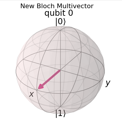
This tool is beneficial in some quantum algorithms since it allows presenting qubits using trigonometric properties that are achieved using the spherical angles.
Quantum Circuit
In the classic world, logic circuits are entities that receive bits and perform logical operators whose outcomes are bit(s). These circuits are composed of logic gates such as XOR , AND or NOT. In order to have a good computational model, we need to develop an analog for quantum computation. We need to develop gates to be used for constructing quantum circuits. What is the nature of such gates? In order to gain some intuition, we observe Bloch sphere.
Recall that we saw that each unit can be presented as a vector on the Bloch sphere, hence qubits have a fixed magnitude. Fixed magnitude as we learned in one of the previous sections is somehow related to unitary matrices. Therefore we have natural candidates for such gates.
Indeed, one can think of a quantum circuit as a chain that receives qubits as inputs, and performs a sequence of unitary operators and measurements. In the following sections, I will present some of the most commonly used gates.
Hadamard Gate
This is probably the most commonly used gate. It is represented by the matrix:
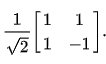
and performs the following maps :
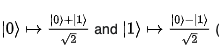
We can view this gate as follows:

The outcome is a qubit that receives 0 and 1 with equal prob
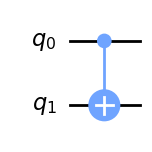
CNOT
A two qubits gate that preserves the second qubit if the first is zero and alters it if it is 1

Phase Shift (U1)
A single qubit gate that rotates |1> in angle ƛ

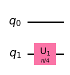
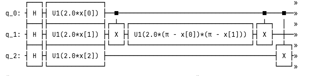
Here is an example circuit:

What does it do?
- It performs a Hadamard gate on each of the initial qubits
- It performs a control not on the second qubit but upon the first
- It rotates the third qubit
- It measures the entire qubits
Avanan’s Actual Examples
We discussed some quantum computation ideas, now it is time to test them on real Avanan data. For this purpose I will present two quantum AI algorithms, the first one is geometric: the quantum version of SVM, and the second is a quantum probabilistic approach to Bayesian networks. Before moving forward I wish to stress that these algorithms are fairly new and that the examples are currently not competitive production-wise but in an early research stage.
What is SVM?
SVM is a classical ML algorithm. It assumes that two (or more ) clusters are separable on a given feature space. The algorithm aims therefore to find the equation of the “wall” that separates these clusters in a way that it leaves the biggest plausible area between the clusters.
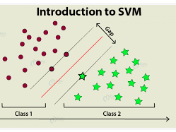
The image above illustrates this process: The planar space in which the stars and dots are located is the features’ space. We assume that the two populations (stars and dots) differ in this space and all is needed is to find an optimal wall (the red line). Nowadays, this method is considered less efficient compared to some new advanced algorithms. Nevertheless, until the appearance of DL, it was a leading method in plenty of research teams ( I personally interviewed candidates that this was the only method that they knew after completing their PhD.)
QVSM
SVM has a quantum analog. Clearly, it requires several modifications both in the data pre-processing as well as in extracting the outcomes. There are several steps that need to be taken:
We need to decide on the number of qubits. As a rule of thumb, we take the data dimension.
We then set a quantum circuit that performs the algorithm.
Finally, we have to set a method for extracting the information.
For SVM we commonly consider kernel issues which in QSVM are taken as a combination of classic functions and which are followed by a unitary operator over their outputs. This mimics the feature extractions steps.
This advantage of QSVM depends on the complexity of these functions. You can read more on the technical details of these steps.
A common approach for this feature extractions is the following:
In the training stage we have two challenges:
- Finding the quantum kernel - Using quantum computation.
- Optimizing the SVM’s weights (this is done using classic manners)
The process that surrounds this training and test is sheer classical training.
Running it on our example (without using too many resources) we got the following separations between clean and phishing emails:
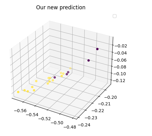
We can see that the separation is not perfect. However, it is good enough for doing further research with additional data
The next graph revalidates my previous statement :

A Probabilistic Approach
The next method relies on an empirical probabilistic approach. We use a set of raw data with some aggregators e.g. binning or special mappings, as features for our engine. This engine aims to estimate the probability that a given email (upon mapping it to its features) is phishing or not. In contrast to QSVM, here we use a single qubit where each of its components |0> and |1> represents a cluster. The quantum algorithm aims to optimize the coefficients in order to achieve a coherent measurement. Recall that a qubit is

Where α and β are complex numbers and the sum of their magnitudes is 1.
USing Bloch sphere properties we have
α= cos(θ2)
β= sin(θ2)
Since we used a real function for preparing the data we can assume that α and β are real, thus phi is taken to be zero.
Observing Bloch sphere for random data, the qubit can be visualized as follow:

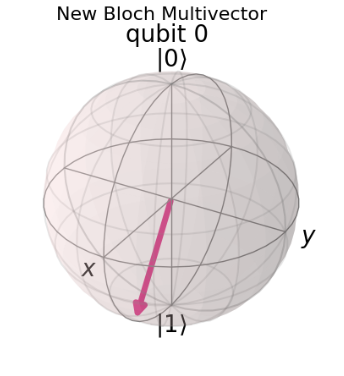
In more informative data, we may obtain the following
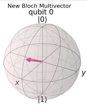
We can see that when the data is more informative the qubit as a vector is located within the upper part of the sphere and not on the x-y plane.
The good news is that our experimental data is even better:
We can summarize the process into three steps:
- Creating a quantum state from the data using a classical code and prior analytics (Parametrized Quantum Circuit -PQC)
- Performing the quantum circuit process based on the quantum state -Quantum comp.
- Taking the measurement for post-process steps such as prediction -Classic
The third step is pretty trivial, whereas the upper steps can be implemented by using various methods. For our example, I use a quantum circuit that merely measures the given quantum state. For creating the state I measure a correlation between each of my features and the target.
Results

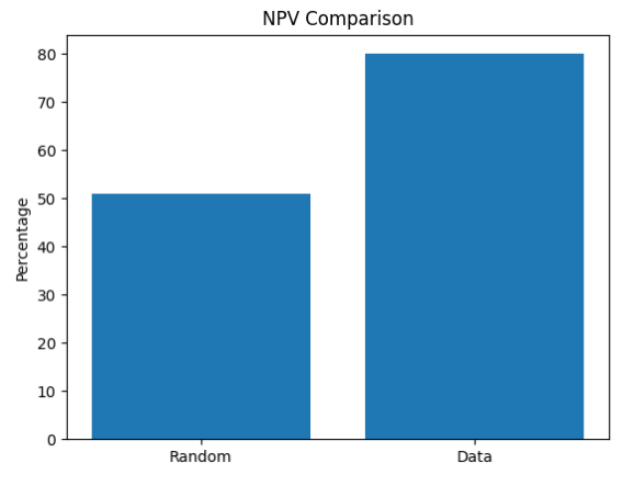
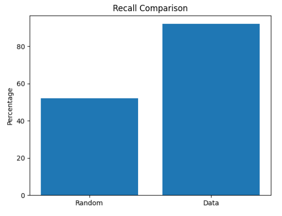
We can see that for three KPIs we improved the prediction using the PQC. The results are not yet commercially competitive but still, it hints that this direction is promising.
Corollary
Quantum computation is an extremely promising computational domain. It can be beneficial for handling problems that are endowed with high complexity. Nevertheless AI- wise it still requires some further research for making it commercially compatible.